Ready to learn Artificial Intelligence? Browse courses like Uncertain Knowledge and Reasoning in Artificial Intelligence developed by industry thought leaders and Experfy in Harvard Innovation Lab.
Welcome to part five of Learning AI if You Suck at Math. If you missed part 1, part 2, part3 and part4 be sure to check them out.
Today, we’re going to write our own Python image recognition program.
To do that, we’ll explore a powerful deep learning architecture called a deep convolutional neural network (DCNN).
Convnets are the workhorses of computer vision. They power everything from self-driving cars to Google’s image search. At TensorFlow Summit 2017, a researcher showed how they’re using a convnet to detect skin cancer as well as a dermatologist with a smart phone!
So why are neural networks so powerful? One key reason:
They do automatic pattern recognition.
So what’s pattern recognition and why do we care if it’s automatic?
Patterns come in many forms but let’s take two critical examples:
- The features that define a physical form
- The steps it takes to do a task
Computer Vision
In image processing pattern recognition is known as feature extraction.
When you look at a photo or something in the real world you’re selectively picking out the key features that allow you to make sense of it. This is something you do unconsciously.
When you see the picture of my cat Dove you think “cat” or “awwwwww” but you don’t really know how you do that. You just do it.
You don’t know how you do it because it’s happening automatically and unconsciously.

My beautiful cat Dove. Your built in neural network knows this is a cat.
It seems simple to you because you do it every day, but that’s because the complexity is hidden away from you.
Your brain is a black box. You come with no instruction manual.
Yet if you really stop to think about it, what you just did in a fraction of second involved a massive number of steps. On the surface it’s deceptively simple but it’s actually incredibly complex.
- You moved your eyes.
- You took in light and you processed that light into component parts which sent signals to your brain.
- Then your brain went to work, doing its magic, converting that light to electro-chemical signals.
- Those signals fired through your built in neural network, activating different parts of it, including memories, associations and feelings.
- At the most “basic” level your brain highlighted low level patterns (ears, whiskers, tail) that it combined into higher order patterns (animal).
- Lastly, you made a classification, which means you turned it into a word, which is a symbolic representation of the real life thing, in this case a “cat.”
All of that happened in the blink of an eye.
If you tried to teach a computer to do that, where would you even begin?
- Could you tell it how to detect ears?
- What are ears?
- How do you describe them?
- Why are cat ears different than human ears or bat ears (or Batman)?
- What do ears look like from various angles?
- Are all cat ears the same (Nope, check out a Scottish Fold)?
The problems go on and on.
If you couldn’t come up with a good answer on how to teach a computer all those steps with some C++ or Python, don’t feel bad, because it stumped computer scientists for 50 years!
What you do naturally is one of the key uses for a deep learning neural network, which is a “classifier”, in this case an image classifier.
In the beginning, AI researchers tried to do the exercise we just went through. They attempted to define all the steps manually. For example, when it comes to natural language processing or NLP, they assembled the best linguists and said “write down all the ‘rules’ for languages.” They called these early AI’s “expert systems.”
The linguists sat down and puzzled out a dizzying array of if, then, unless, except statements:
- Does a bird fly?
Yes
Unless it’s:
- Dead
- Injured
- A flightless bird like a Penguin
- Missing a wing
These lists of rules and exceptions are endless. Unfortunately they’re also terribly brittle and prone to all kinds of errors. They’re time consuming to create, subject to debate and bias, hard to figure out, etc.
Deep neural networks represent a real breakthrough because instead of you having to figure out all the steps, you can let the machine extract thekey features of a cat automatically.
“Automatically” is essential because we bypass the impossible problem of trying to figure out all those thousands or millions of hidden steps we take to do any complex action.
We can let the computer figure it out for itself!
The Endless Steps of Everything
Let’s look at the second example: Figuring out the steps to do a task.
Today we do this manually and define the steps for a computer. It’s called programming. Let’s say you want to find all the image files on your hard drive and move them to a new folder.
For most tasks the programmer is the neural network. He’s the intelligence. He studies the task, decomposes it into steps and then defines each step for the computer one by one. He describes it to the computer with a symbolic representation known as a computer programming language.
Here’s an example in Python, from “Jolly Jumper” on Stack Exchange:
importshutil
import os
dst_dir = “your/destination/dir”
shutil.move(jpgfile, dst_dir)
Jolly Jumper figured out all the steps and translated them for the computer, such as:
- We need to know the source directory
- Also, we need a destination
- We need a way of classifying the types of files we want, in this case a “jpg” file
- Lastly we go into the directory, search it for any jpgs and move them from the source to the destination directory
This works well for simple and even moderately complex problems. Operating systems are some of the most complex software on Earth, composed of 100’s of millions of lines of code. Each line is an explicit instruction for how computers do tasks ( like draw things on the screen, store and update information ) as well as how people do tasks ( copy files, input text, send email, view photos, chat with others, etc. ).
But as we evolve to try and solve more challenging problems we’re running into the limits of our ability to manually define the steps of the problem.
For example, how do you define driving a car?
There are hundreds of millions of tiny steps that we take to do this mind-numbingly complex task. We have to:
- Stay in the lines
- Know what a line is and be able to recognize it
- Navigate from one place to another
- Recognize obstructions like walls, people, debris
- Classify objects as helpful (street sign) or threat (pedestrian crossing a green light)
- Assess where all the drivers around us are constantly
- Make split second decisions
In machine learning this is known as a decision making problem. Examples of complex decision making problems are:
- Robot navigation and perception
- Language translation systems
- Self driving cars
- Stock trading systems
The Secret Inner Life of Neural Networks
Let’s see how deep learning helps us solve the insane complexity of the real world by doing automatic feature extraction!
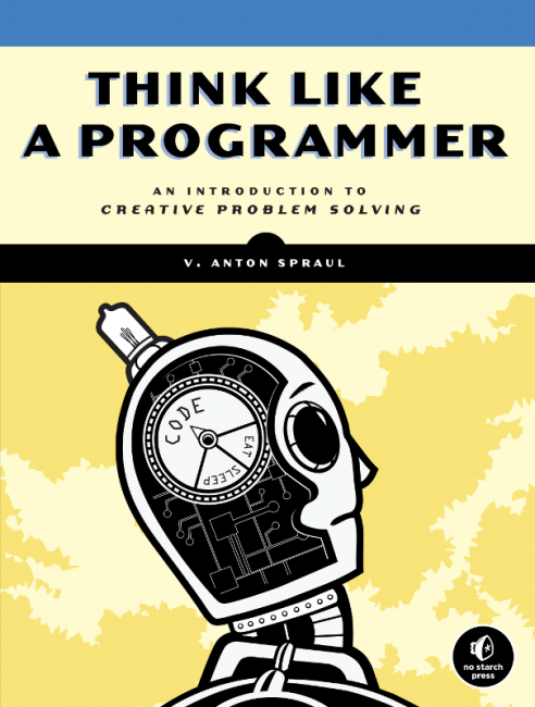
If you’ve ever read the excellent book Think Like a Programmer, by V. Anton Spraul (and you should), you know that programming is about problem solving. The programmer decomposes a problem down into smaller problems, creates an action plan to solve it and then writes code to make it happen.
Deep Learning solves problems for us, but AI still needs humans at this point (thank God) to design and test AI architectures (at least for now.) So let’s decompose a neural net into its parts and build a program to recognize that the picture of my Dove is a cat.
The Deep in Deep Learning
Deep learning is subfield of machine learning. It’s name comes from the idea that we stack together a bunch of different layers to learn increasingly meaningful representations of data.
Each of those layers are neural networks, which consist of linked connections between artificial neurons.
Before we had powerful GPUs to do the math for us we could only build very small “toy” neural nets. They couldn’t do very much. Today we can stack many layers together hence the “deep” in deep learning.
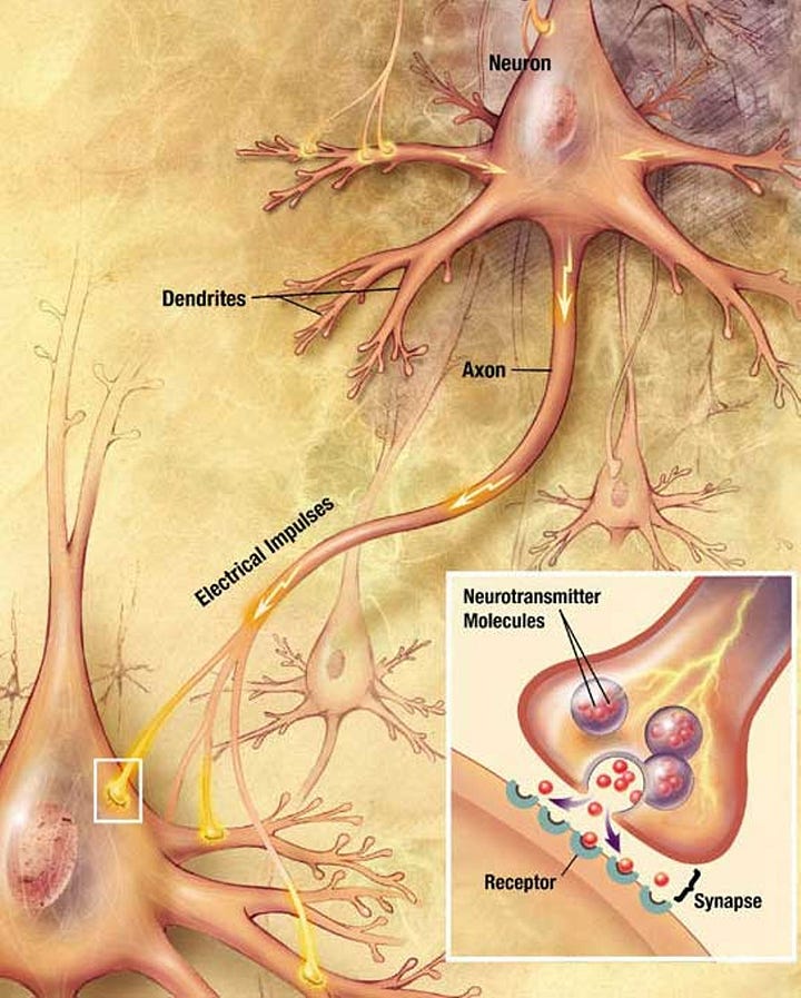
Neural nets were inspired by biological research into the human brain in the 1950s. Researchers created a mathematical representation of a neuron, which you can see below (courtesy of the awesome open courseware on Convolutional Neural Nets from Stanford and Wikimedia Commons):
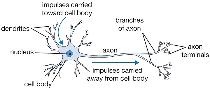
Biological neuron
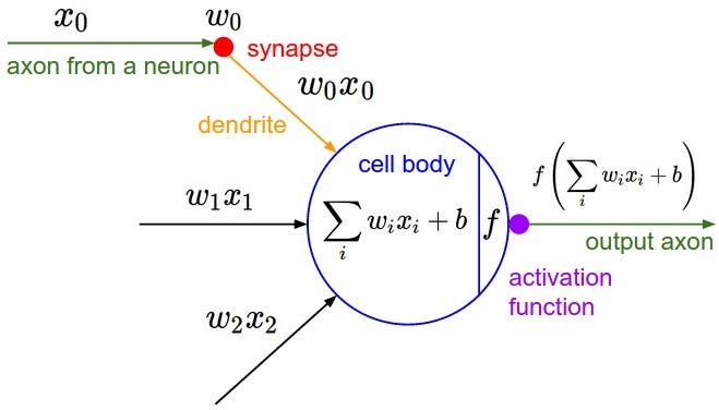
Math model of a neuron.
Forget about all the more complex math symbols for now, because you don’t need them.
The basics are super simple. Data, represented by x0, travels through the connections between the neurons. The strength of the connections are represented by their weights (w0x0, w1x1, etc). If the signal is strong enough, it fires the neuron via its “activation function” and makes the neuron “active.”
Here is an example of a three layer deep neural net:
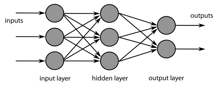
By activating some neurons and not others and by strengthening the connections between neurons, the system learns what’s important about the world and what’s not.
Building and Training a Neural Network
Let’s take a deeper look at deep learning and write some code as we go. All the code is available on my Github here.
The essential characteristics of the system are:
- Training
- Input data
- Layers
- Weights
- Targets
- Loss function
- Optimizer function
- Predictions
Training
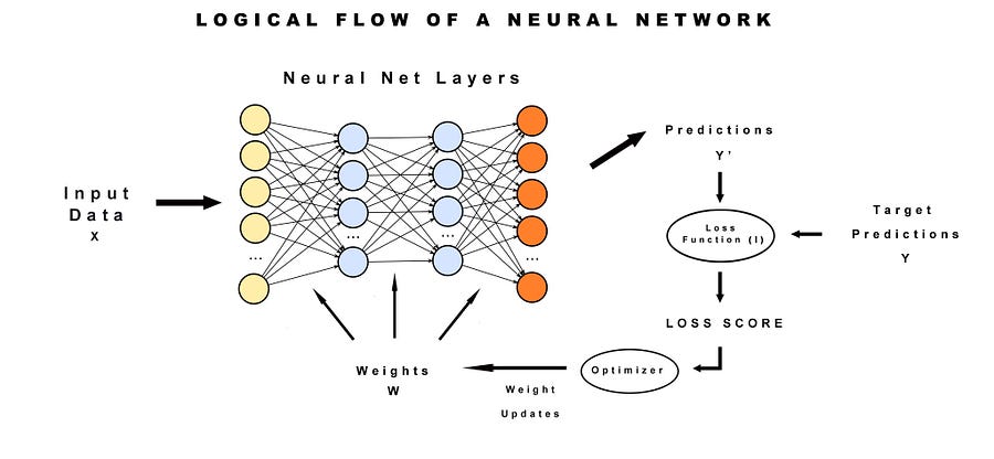
Training is how we teach a neural network what we want it to learn. It follows a simple five step process:
- Create a training data set, which we will call x and load its labels as targets y
- Feed the x data forward through the network with the result being predictions y’
- Figure out the “loss” of the network, which is the difference between the predictions y’ and the correct targets y
- Compute the “gradient” of the loss (l) and which tells us how fast we’re moving towards or away from the correct targets
- Adjust the weights of the network in the opposite direction of the gradient and go back to step two to try again
Input Data
In this case the input data to a DCNN is a bunch of images. The more images the better. Unlike people, computers need a lot of examples to learn how to classify them. AI researchers are working on ways to learn with a lot less data but that’s still a cutting edge problem.
A famous example is the ImageNet data set. It consists of lots of hand labeled images. In other words, they crowd sourced the humans to use their built in neural nets to look at all the images and provide meaning to the data. People uploaded their photos and labeled it with tags, like “dog”, or a specific type of dog like a “Beagle.”
Those labels represent accurate predictions for the network. The closer the network gets to matching the hand labeled data (y) with their predictions (y’) the more accurate the network grows.
The data is broken into two pieces, a training set and testing set. The training set is the input that we feed to our neural network. It learns the key features of various kinds of objects and then we test whether it can accurately find those objects on random data in the test image set.
In our program we’ll use the well known CIFAR-10 dataset which was developed by the Canadian Institute for Advanced Research.
CIFAR-10 has 60000 32×32 color images in 10 classes, with 6000 images per class. We get 50000 training images and 10000 test images.
When I first started working with CIFAR I mistakenly assumed it would be an easier challenge than working with the larger images of the ImageNet challenge. It turns out CIFAR10 is more challenging because the images are so tiny and there are a lot less of them, so they have less identifiable characteristics for our neural network to lock in on.
While some of the biggest and baddest DCNN architectures like ResNet can hit 97% accuracy on ImageNet, it can only hit about 87% on CIFAR 10, in my experience. The current state of the art on CIFAR 10 is DenseNet, which can hit around 95% with a monstrous 250 layers and 15 million parameters! I link to those frameworks at the bottom of the article for further exploration. But it’s best to start with something simpler before diving into those complex systems.
Enough theory! Let’s write code.
If you’re not comfortable with Python, I highly, highly, highly recommend Learning Python by Fabrizio Romano. This book explains everything so well. I’ve never found a better Python book and I have a bunch of them that failed to teach me much.
The code for our DCNN is based on the Keras example code on Github.
You can find my modifications here.
I’ve adjusted the architecture and parameters, as well as added TensorBoard to help us visualize the network.
Let’s initialize our Python program, import the dataset and the various classes we’ll need to build our DCNN. Luckily, Keras already knows how to get this dataset automatically so we don’t have too much work to do.
importnumpy as np
fromkeras.callbacks import TensorBoard
fromkeras.models import Sequential
fromkeras.layers import Dense, Dropout, Activation, Flatten
fromkeras.layers import Convolution2D, MaxPooling2D
fromkeras.utils import np_utils
fromkeras import backend as K
Our neural net starts off with a random configuration. It’s as good a starting place as any but we shouldn’t expect it to start off very smart. Then again, it’s possible that some random configuration gives us amazing results completely by accident, so we seed the random weights to make sure that we don’t end up with state of the art results by sheer dumb luck!
np.random.seed(1337) # Very l33t
Layers
Now we’ll add some layers.
Most neural networks use fully connected layers. That means they connect every neuron to every other neuron.
Fully connected layers are fantastic for solving all kinds of problems. Unfortunately they don’t scale very well for image recognition.
So we’ll build our system using convolutional layers, which are unique because they don’t connect all the neurons together.
Let’s see what the Stanford course on computer vision has to say about convnet scaling:
“In CIFAR-10, the image are merely 32x32x3 (32 wide, 32 high, 3 color channels), so a single fully-connected neuron in a first hidden layer of a regular Neural Network would have 32*32*3 = 3072 weights. This amount still seems manageable, but clearly this fully-connected structure does not scale to larger images. For example, an image of more respectible size, e.g. 200x200x3, would lead to neurons that have 200*200*3 = 120,000 weights. Moreover, we would almost certainly want to have several such neurons, so the parameters would add up quickly! Clearly, this full connectivity is wasteful and the huge number of parameters would quickly lead to overfitting.”
Overfitting is when you train the network so well that it kicks ass on the training data but sucks when you show it images it’s never seen. In other words it’s not much use in the real world.
It’s as if you played the same game of chess over and over and over again until you had it perfectly memorized. Then someone makes a different move in a real game and you have no idea what to do. We’ll look at overfitting more later.
Here’s how data flows through a DCNN. It looks at only a small subset of the data, hunting for patterns. It then builds those observations up into higher order understandings.
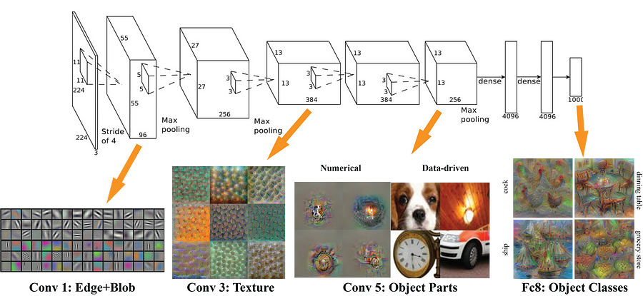
A visual representation of a convolutional neural net from the mNeuron plugin created for MIT’s computer vision courses/teams.
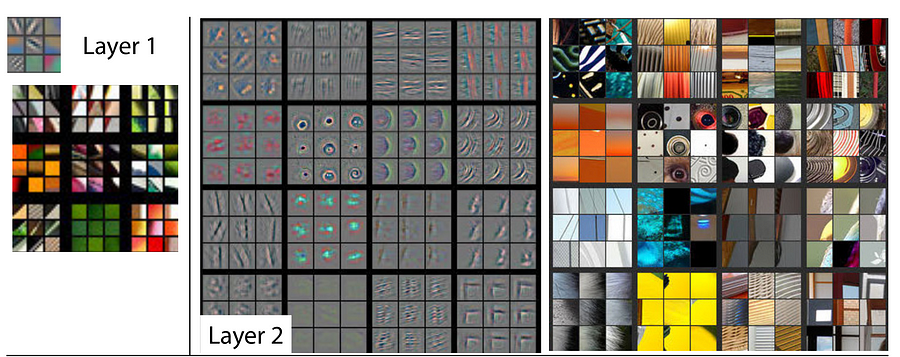
Notice how the first few layers are simple patterns like edges and colors and basic shapes.
As the information flows through the layers, the system finds more and more complex patterns, like textures, and eventually it deduces various object classes.
The ideas were based on experiments on cat vision that showed that different cells responded to only certain kinds of stimuli such as an edge or a particular color.
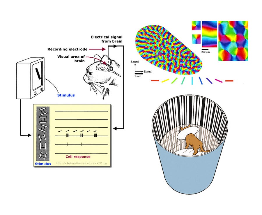
Slides from the excellent Deep Learning open course at Oxford.
The same is true for humans. Our visual cells respond only to very specific features.
Here is a typical DCNN architecture diagram:
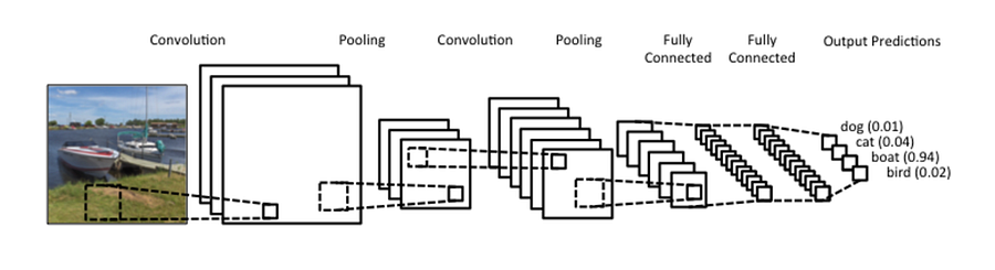
You’ll notice a third kind of layer in there, a pooling layer. You can find all kinds of detail in the Oxford lectures and the Standford lectures. However, I’m going to skip a lot of the granular detail because most people just find it confusing. I know I did when I first tried to make sense of it.
Here’s what you need to know about pooling layers. Their goal is simple. They do subsampling. In other words they shrink the input image, which reduces the computational load and memory usage. With less information to crunch we can work with the images more easily.
They also help reduce a second kind of overfitting where the network zeros in on anomalies in the training set that really have nothing to do with picking out dogs or birds or cats. For example, there may be some garbled pixels or some lens flares on a bunch of the images. The network may then decide that lens flare and dog go together, when they’re about as closely related as an asteroid and a baby rattle.
Lastly, most DCNNs add a few densely connected, aka fully connected layers to process out all the features maps detected in earlier layers and make predictions.
So let’s add a few layers to our convnet.
First we add some variables that we will pull into our layers.
batch_size = 128
nb_classes = 10
nb_epoch = 45
img_rows, img_cols = 32, 32
nb_filters = 32
pool_size = (2, 2)
# convolution kernel size
kernel_size = (3, 3)
The kernel and pooling size define how the convolutional network passes over the image looking for features. The smallest kernel size would be 1×1, which means we think key features are only 1 pixel wide. Typical kernel sizes check for useful features over 3 pixels at a time and then pool those features down to a 2×2 grid.
The 2×2 grid pulls the features out of the image and stacks them up like trading cards. This disconnects them from a specific spot on the image and allows the system to look for straight lines or swirls anywhere, not just in the spot it found them in the first place.
Most tutorials describe this as dealing with “translation invariance.”
What the heck does that mean? Good question.
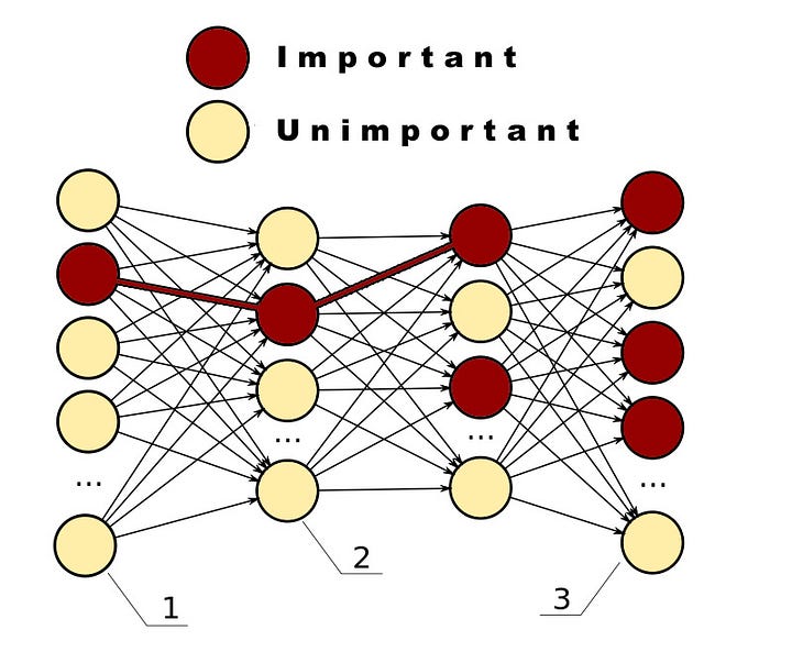
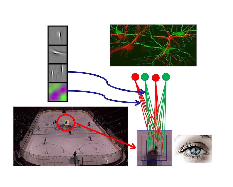
Take a look at this image again:
Without yanking the features out, like you see in layer 1 or layer 2, the system might decide that the circle of a cat’s nose was only important right smack in the center of the image where it found it.
Let’s see how that works with my Dove. If the system originally finds a circle in her eye then it might mistakenly assume that the position of the circle in an image is relevant to detecting cats.

Instead the system should look for circles wherever they may roam, as we see below.

Before we can add the layers we need to load and process the data.
X_train = X_train.reshape(X_train.shape[0], 3, img_rows, img_cols)
X_test = X_test.reshape(X_test.shape[0], 3, img_rows, img_cols)
input_shape = (1, img_rows, img_cols)
else:
X_train = X_train.reshape(X_train.shape[0], img_rows, img_cols, 3)
X_test = X_test.reshape(X_test.shape[0], img_rows, img_cols, 3)
input_shape = (img_rows, img_cols, 3)
X_test = X_test.astype(‘float32’)
X_train /= 255
X_test /= 255
print(‘X_train shape:’, X_train.shape)
print(X_train.shape[0], ‘train samples’)
print(X_test.shape[0], ‘test samples’)
Y_test = np_utils.to_categorical(y_test, nb_classes)
border_mode=’valid’,
input_shape=input_shape))
model.add(Activation(‘relu’))
model.add(Convolution2D(nb_filters, kernel_size[0], kernel_size[1]))
model.add(Activation(‘relu’))
model.add(MaxPooling2D(pool_size=pool_size))
model.add(Dropout(0.25))
The layers are stacked as follows:
- Convolution
- Activation
- Convolution
- Activation
- Pooling
- Dropout
We’ve already discussed most of these layer types except for two of them, dropout and activation.
Dropout is the easiest to understand. Basically it’s a percentage of how much of the model to randomly kill off. This is similar to how Netflix uses Chaos Monkey. They have scripts that turn off random servers in their network to ensure the network can survive with its built in resilience and redundancy. The same is true here. We want to make sure the network is not too dependent on any one feature.
The activation layer is a way to decide if the neuron “fires” or gets “activated.” There are dozens of activation functions at this point. RELU is the one of the most successful because of its computational efficiency. Here is a list of all the different kinds of activation functions available in Keras.
We’ll also add a second stack of convolutional layers that mirror the first one. If we were rewriting this program for efficiency we would create a model generator and do a for loop to create however many stacks we want. But in this case we will just cut and paste the layers from above, violating the zen rules of Python for expediency sake.
model.add(Activation(‘relu’))
model.add(Convolution2D(nb_filters, kernel_size[0], kernel_size[1]))
model.add(Activation(‘relu’))
model.add(MaxPooling2D(pool_size=pool_size))
model.add(Dropout(0.25))
Lastly, we add the dense layers, some more drop out layers and we flatten all the features maps.
model.add(Dense(256))
model.add(Activation(‘relu’))
model.add(Dropout(0.5))
model.add(Dense(nb_classes))
model.add(Activation(‘softmax’))
We use a different kind of activation called softmax on the last layer, because it defines a probability distribution over the classes.
Weights
We talked briefly about what weights were earlier but now we’ll look at them in depth.
Weights are the strength of the connection between the various neurons.
We have parallels for this in our own minds. In your brain, you have a series of biological neurons. They’re connected to other neurons with electrical/chemical signals passing between them.
But the connections are not static. Over time some of those connections get stronger and some weaker.
The more electro-chemical signals flowing between two biological neurons, the stronger those connections get. In essence, your brain rewires itself constantly as you have new experiences. It encodes your memories and feelings and ideas about those experiences by strengthening the connections between some neurons.
Source U.S. National Institute of Health — Wikimedia Commons.
Computer based neural networks are inspired by biological ones. We call them Artificial Neural Networks or ANNs for short. Usually when we say “neural network” what we really mean is ANN. ANN’s don’t function exactly the same as biological ones, so don’t make the mistake of thinking an ANN is some kind of simulated brain. It’s not. For example in a biological neural network (BNN), every neuron does not connect to every other neuron whereas in an ANN every neuron in one layer generally connects to every neuron in the next layer.
Below is an image of a BNN showing connections between various neurons. Notice they’re not all linked.

Source: Wikimedia Commons: Soon-Beom HongAndrew ZaleskyLuca CocchiAlex FornitoEun-Jung ChoiHo -Hyun KimJeong -Eun SuhChang-Dai KimJae -Won KimSoon -Hyung Yi
Though there are many differences, there are also very strong parallels between BNNs and ANNs.
Just like the neurons in your head form stronger or weaker connections, the weights in our artificial neural network define the strength of the connections between neurons. Each neuron knows a little bit about the world. Wiring them together allows them to have a more comprehensive view of the world when taken together. The ones that have stronger connections are considered more important for the problem we’re trying to solve.
Let’s look at several screenshots of the Neural Network Playground, a visualizer for TensorFlow to help understand this better.
The first network shows a simple six layer system. What the network is trying to do is cleanly separate the blue dots from the orange dots in the picture on the far right. It’s looking for the best pattern that separates them with a high degree of accuracy.
I have not yet started training the system here. Because of that we can see weights between neurons are mostly equal. The thin dotted lines are weak connections and the thicker lines are strong connections. The network is initialized with random weights as a starting point.
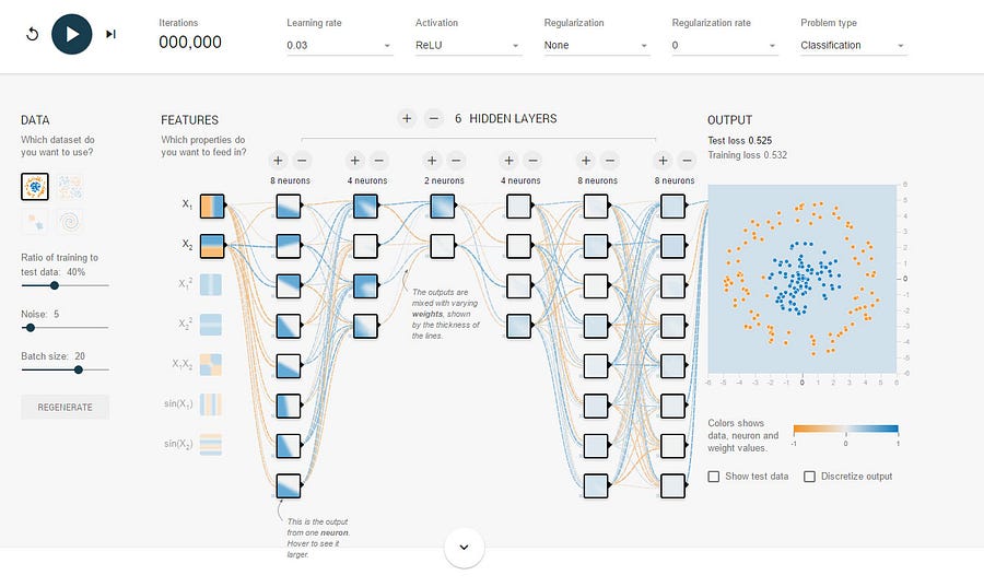
Now let’s take a look at the network after we’ve trained it.
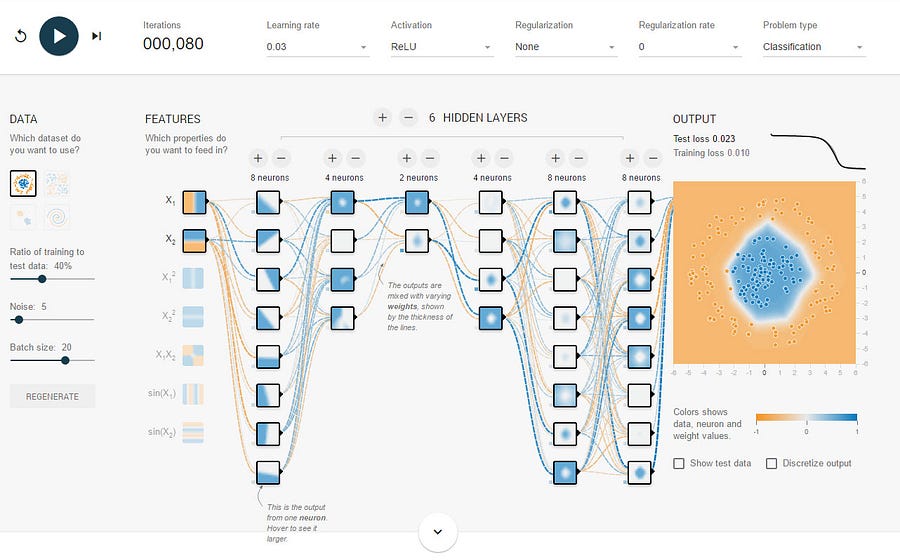
First notice the picture on the far right. It now has a nice blue dot in the middle around the blue dots and orange around the rest of the picture. As you can see it’s done pretty well, with a high degree of accuracy. This happened over 80 “epochs” or training rounds.
Also notice that many of the weights have strong blue dotted lines between various neurons. The weights have increased and now the system is trained and ready to take on the world!
Training Our Neural Net and Optimizing It
Now let’s have the model crunch some numbers. To do that we compile it and set its optimizer function.
optimizer=’adam’,
metrics=[‘accuracy’])
It took me a long time to understand the optimizer function because I find most explanations miss the “why” behind the “what.”
In other words, why the heck do I need an optimizer?
Remember that a network has target predictions y and as it’s trained over many epochs it makes new predictions y’. The system tests these predictions against a random sample from the test dataset and that determines the system’s validation accuracy. A system can end up 99% accurate on the training data and only hit 50% or 70% on test images, so the real name of the game is validation accuracy, not accuracy.
The optimizer calculates the gradient (also known as partial derivatives in math speak) of the error function with respect to the model weights.
What does that mean? Think of the weights distributed across a 3D hilly landscape (like you see below), which is called the “error landscape.” The “coordinates” of the landscape represent specific weight configurations (like coordinates on a map), while the “altitude” of the landscape corresponds to the total error/cost for the different weight configurations.
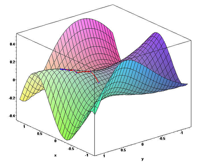
Error landscape
The optimizer serves one important function. It figures out how to adjust the weights to try to minimize the errors. It does this by taking a page from the book of calculus.
What is calculus? Well if you turn to any math text book you’ll find some super unhelpful explanations such as it’s all about calculating derivatives or differentials. But what the heck does that mean?

I didn’t understand it until I read Calculus Better Explained, by Kalid Azad.
Here’s what nobody bothers to explain.
Calculus does two things:
- Breaks things down into smaller chunks, aka a circle into rings.
- Figures out rates of change.
In other words if I slice up a circle into rings:
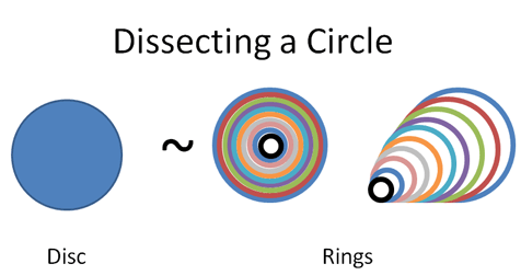
Courtesy of the awesome Calculus Explained website.
I can unroll the rings to do some simple math on it:
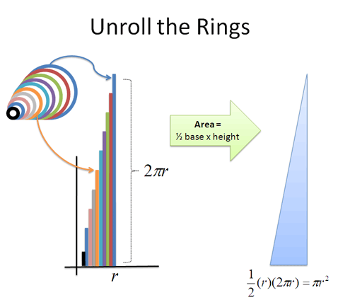
Bam!
In our case we run a bunch of tests, adjust the weights of the network but did we actually get any closer to an better solution to the problem? The optimizer tells us that!
You can read about gradient descent with an incredible amount of detail here or in the Stanford course but you’ll probably find like I did that they’re long on detail and light on the crucial question of why.
In essence, what you’re trying to do is minimize the errors. It’s a bit like driving around in the fog. In an earlier version of this post, I characterized gradient descent as a way to to find an optimal solution. But actually, there is really no way to know if we have an “optimal” solution at all. If we knew what that was, we would just go right to it. Instead we are trying to find a “better” solution that works. This is a bit like evolution. We find something that is fit enough to survive but that doesn’t mean we created Einstein!
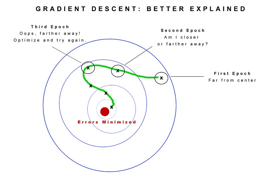
Think of gradient descent like when you played Marco Polo as a kid.
You closed your eyes and all your friends spread out in the pool. You shouted out “Marco” and all the kids had to answer “Polo.” You used your ears to figure if you were getting closer or farther away. If you were farther away you adjusted and tried a different path. If you were closer you kept going in that direction. Here we’re figuring out how best to adjust the weights of the network to help them get closer to understanding the world.
We chose the “adam” optimizer described in this paper. I’ve found through brute force changing my program that it seems to produce the best results. This is the art of data science. There is no one algorithm to rule them all. If I changed the architecture of the network, I might find a different optimizer worked better.
Here is a list of all the various optimizers in Keras.
Next we set up TensorBoard so we can visualize how the network performs.
tb = TensorBoard(log_dir=’./logs’)
All we did was create a log directory. Now we will train the model and point TensorBoard at the logs.
print(“Accuracy: %.2f%%” % (score[1]*100))
All right, let’s fire this bad boy up and see how it does!
Epoch 89/100
50000/50000 [==============================] – 3s – loss: 0.4834 – acc: 0.8269 – val_loss: 0.6286 – val_acc: 0.7911
Epoch 90/100
50000/50000 [==============================] – 3s – loss: 0.4908 – acc: 0.8224 – val_loss: 0.6169 – val_acc: 0.7951
Epoch 91/100
50000/50000 [==============================] – 4s – loss: 0.4817 – acc: 0.8238 – val_loss: 0.6052 – val_acc: 0.7952
Epoch 92/100
50000/50000 [==============================] – 4s – loss: 0.4863 – acc: 0.8228 – val_loss: 0.6151 – val_acc: 0.7930
Epoch 93/100
50000/50000 [==============================] – 3s – loss: 0.4837 – acc: 0.8255 – val_loss: 0.6209 – val_acc: 0.7964
Epoch 94/100
50000/50000 [==============================] – 4s – loss: 0.4874 – acc: 0.8260 – val_loss: 0.6086 – val_acc: 0.7967
Epoch 95/100
50000/50000 [==============================] – 3s – loss: 0.4849 – acc: 0.8248 – val_loss: 0.6206 – val_acc: 0.7919
Epoch 96/100
50000/50000 [==============================] – 4s – loss: 0.4812 – acc: 0.8256 – val_loss: 0.6088 – val_acc: 0.7994
Epoch 97/100
50000/50000 [==============================] – 3s – loss: 0.4885 – acc: 0.8246 – val_loss: 0.6119 – val_acc: 0.7929
Epoch 98/100
50000/50000 [==============================] – 3s – loss: 0.4773 – acc: 0.8282 – val_loss: 0.6243 – val_acc: 0.7918
Epoch 99/100
50000/50000 [==============================] – 3s – loss: 0.4811 – acc: 0.8271 – val_loss: 0.6201 – val_acc: 0.7975
Epoch 100/100
50000/50000 [==============================] – 3s – loss: 0.4752 – acc: 0.8299 – val_loss: 0.6140 – val_acc: 0.7935
Test score: 0.613968349266
Accuracy: 79.35%
We hit 79% accuracy after 100 epochs. Not bad for a few lines of code. Now you might think 79% is not that great, but remember that in 2011, that was better than state of the art on Imagenet and it took a decade to get there! And we did that with just some example code from the Keras Github and a few tweaks.
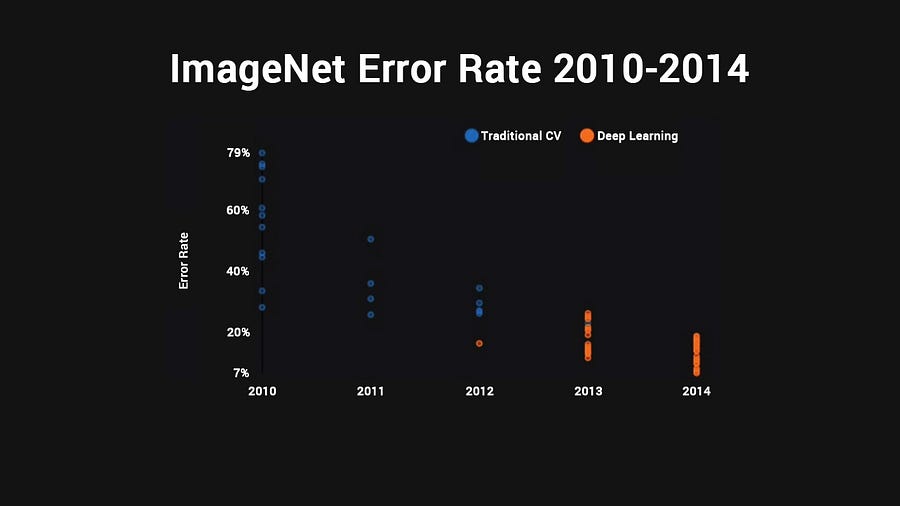
You’ll notice that in 2012 is when new ideas started to make an appearance.
AlexNet, by AI researchers Alex Krizhevsky, Ilya Sutskever and Geoffrey Hinton, is the first orange dot. It marked the beginning of the current renaissance in deep learning. By the next year everyone was using deep learning. By 2014 the winning architecture was better than human level image recognition.
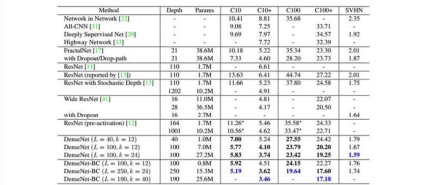
Even so, these architectures are often very tied to certain types of problems. Several of the most popular architectures today, like ResNet and Google’s Inception V3 do only 88% on the tiny CIFAR10 images. They do even worse on the larger CIFAR100 set.
The current state of the art is DenseNet, which won the ImageNet contest last year in 2016. It chews through CIFAR10, hitting a killer 94.81% accuracywith an insanely deep 250 layers and 15.3 million connections! It is an absolute monster to run. On a single Nvidia 1080GTX, if you run it with the 40 x 12 model which hits the 93% accuracy mark you see in the chart below, it will take a month to run. Ouch!
That said, I encourage you to explore these models in depth to see what you can learn from them.
I did some experimenting and managed to hack together a weird architecture through brute force experimentation that achieve 81.40% accuracy using nothing but the build in Keras layers and no custom layers. You can find that on Github here.
50000/50000 [==============================] – 10s – loss: 0.3503 – acc: 0.8761 – val_loss: 0.6229 – val_acc: 0.8070
Epoch 71/75
50000/50000 [==============================] – 10s – loss: 0.3602 – acc: 0.8740 – val_loss: 0.6039 – val_acc: 0.8085
Epoch 72/75
50000/50000 [==============================] – 10s – loss: 0.3543 – acc: 0.8753 – val_loss: 0.5986 – val_acc: 0.8094
Epoch 73/75
50000/50000 [==============================] – 10s – loss: 0.3461 – acc: 0.8780 – val_loss: 0.6052 – val_acc: 0.8147
Epoch 74/75
50000/50000 [==============================] – 10s – loss: 0.3418 – acc: 0.8775 – val_loss: 0.6457 – val_acc: 0.8019
Epoch 75/75
50000/50000 [==============================] – 10s – loss: 0.3440 – acc: 0.8776 – val_loss: 0.5992 – val_acc: 0.8140
Test score: 0.599217191744
Accuracy: 81.40%
We can load up TensorBoard to visualize how we did as well.
tensorboard --logdir=./logs
Now open a browser and go to the following URL:
127.0.1.1:6006
Here is a screenshot of the training over time.
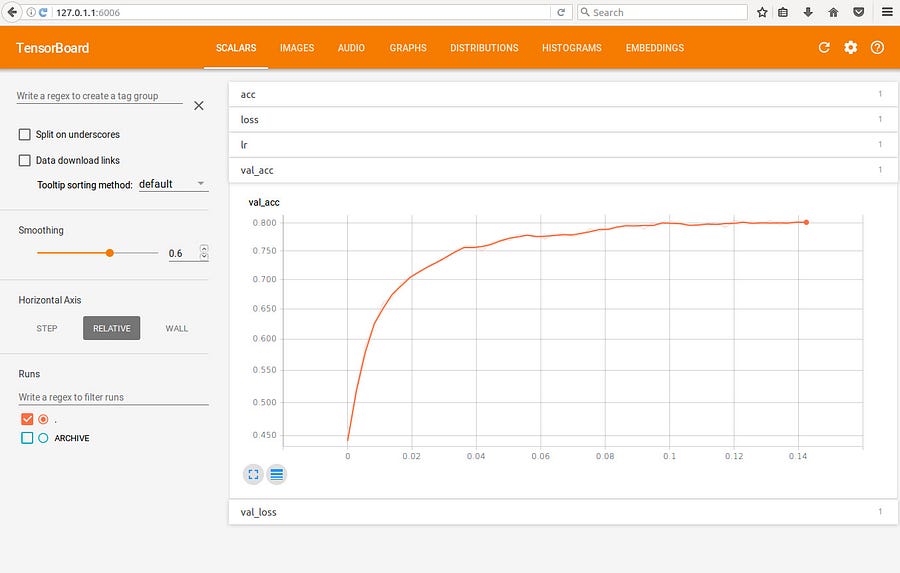
You can see we quickly start to pass the point of diminishing returns at around 35 epochs and 79%. The rest of the time is spent getting it to 81.40% and likely overfitting at anything beyond 75 epochs.
So how would you improve this model?
Here are a few strategies:
- Implement your own custom layers
- Do image augmentation, like flipping images, enhancing them, warping them, cloning them, etc
- Go deeper
- Change the settings on the layers
- Read through the winning architecture papers and stack up your own model that has similar characteristics
And thus you have reached the real art of data science, which is using your brain to understand the data and hand craft a model to understand it better. Perhaps you dig deep into CIFAR10 and notice that upping the contrast on those images would really make images stand out. Do it!
Don’t be afraid to load things up in Photoshop and start messing with filters to see if images get sharper and clearer. Figure out if you can do the same thing with Keras image manipulation functions.
Deep learning is far from a magic bullet. It requires patience and dedication to get right.
It can do incredible things but you may find yourself glued to your workstation watching numbers tick by for hours until 2 in the morning, getting absolutely nowhere.
But then you hit a breakthrough!
It’s a bit like the trial and error a neural net goes through. Try some stuff, get closer to an answer. Try something else and get farther away.
I am now exploring how to use genetic algorithms to auto-evolve neural nets. There’s been a bunch of work done on this front but not enough!
Eventually we’ll hit a point where many of the architectures are baked and easy to implement by pulling in some libraries and some pre-trained weights files but that is a few years down the road for enterprise IT.
This field is still fast developing and new ideas are coming out every day. The good news is you are on the early part of the wave. So get comfortable and start playing around with your own models.
Study. Experiment. Learn.
Do that and you can’t go wrong.