
Ready to learn Machine Learning? Browse courses like Machine Learning Foundations: Supervised Learning developed by industry thought leaders and Experfy in Harvard Innovation Lab.

Photo Credit: Pixabay
Apache Spark, once a component of the Hadoop ecosystem, is now becoming the big-data platform of choice for enterprises. It is a powerful open source engine that provides real-time stream processing, interactive processing, graph processing, in-memory processing as well as batch processing with very fast speed, ease of use and standard interface.
In the industry, there is a big demand for a powerful engine that can do all of above. Sooner or later, your company or your clients will be using Spark to develop sophisticated models that would enable you to discover new opportunities or avoid risk. Spark is not hard to learn, if you already known Python and SQL, it is very easy to get started. Let’s give it a try today!
Exploring The Data
We will use the same data set when we built a Logistic Regression in Python, and it is related to direct marketing campaigns (phone calls) of a Portuguese banking institution. The classification goal is to predict whether the client will subscribe (Yes/No) to a term deposit. The dataset can be downloaded from Kaggle.
from pyspark.sql import SparkSession
spark = SparkSession.builder.appName(‘ml-bank’).getOrCreate()
df = spark.read.csv(‘bank.csv’, header = True, inferSchema = True)
df.printSchema()
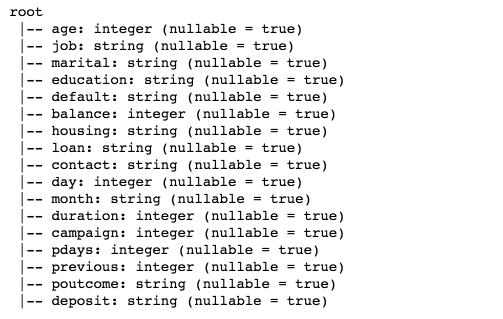
Figure 1
Input variables: age, job, marital, education, default, balance, housing, loan, contact, day, month, duration, campaign, pdays, previous, poutcome.
Output variable: deposit
Have a peek of the first five observations. Pandas data frame is prettier than Spark DataFrame.show().
import pandas as pd
pd.DataFrame(df.take(5), columns=df.columns).transpose()
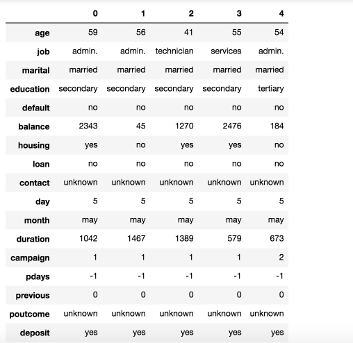
Figure 2
Our classes are perfect balanced.
import pandas as pd
pd.DataFrame(df.take(5), columns=df.columns).transpose()
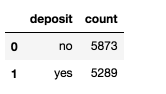
Figure 3
Summary statistics for numeric variables
numeric_features = [t[0] for t in df.dtypes if t[1] == ‘int’]
df.select(numeric_features).describe().toPandas().transpose()
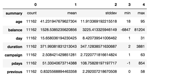
Figure 4
Correlations between independent variables.
numeric_data = df.select(numeric_features).toPandas()
axs = pd.scatter_matrix(numeric_data, figsize=(8, 8));
n = len(numeric_data.columns)
for i in range(n):
v = axs[i, 0]
v.yaxis.label.set_rotation(0)
v.yaxis.label.set_ha(‘right’)
v.set_yticks(())
h = axs[n-1, i]
h.xaxis.label.set_rotation(90)
h.set_xticks(())
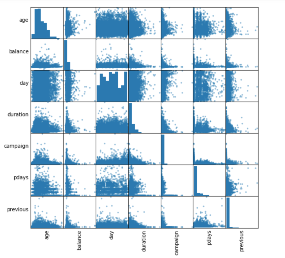
Figure 5
It’s obvious that there aren’t highly correlated numeric variables. Therefore, we will keep all of them for the model. However, day and month columns are not really useful, we will remove these two columns.
cols = df.columns
df.printSchema()
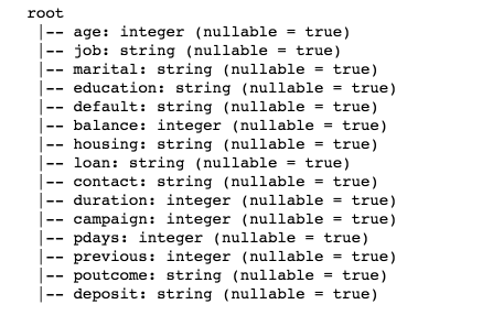
Figure 6
Preparing Data for Machine Learning
The process includes Category Indexing, One-Hot Encoding and VectorAssembler — a feature transformer that merges multiple columns into a vector column.
from pyspark.ml.feature import OneHotEncoderEstimator,
StringIndexer, VectorAssembler
categoricalColumns = [‘job’, ‘marital’, ‘education’, ‘default’,
‘housing’, ‘loan’, ‘contact’, ‘poutcome’]
stages = []
for categoricalCol in categoricalColumns:
stringIndexer = StringIndexer(inputCol = categoricalCol,
outputCol = categoricalCol + ‘Index’)
encoder = OneHotEncoderEstimator(inputCols=
[stringIndexer.getOutputCol()], outputCols=[categoricalCol +
“classVec”])
stages += [stringIndexer, encoder]
label_stringIdx = StringIndexer(inputCol = ‘deposit’, outputCol = ‘label’)
stages += [label_stringIdx]
numericCols = [‘age’, ‘balance’, ‘duration’, ‘campaign’, ‘pdays’,
‘previous’]
assemblerInputs = [c + “classVec” for c in categoricalColumns] +
numericCols
assembler = VectorAssembler(inputCols=assemblerInputs,
outputCol=”features”)
stages += [assembler]
The above code are taken from databricks’ official site and it indexes each categorical column using the StringIndexer, then converts the indexed categories into one-hot encoded variables. The resulting output has the binary vectors appended to the end of each row. We use the StringIndexer again to encode our labels to label indices. Next, we use the VectorAssembler to combine all the feature columns into a single vector column.
Pipeline
We use Pipeline to chain multiple Transformers and Estimators together to specify our machine learning workflow. A Pipeline’s stages are specified as an ordered array.
from pyspark.ml import Pipeline
pipeline = Pipeline(stages = stages)
pipelineModel = pipeline.fit(df)
df = pipelineModel.transform(df)
selectedCols = [‘label’, ‘features’] + cols
df = df.select(selectedCols)
df.printSchema()
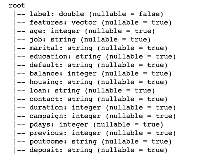
Figure 7
pd.DataFrame(df.take(5), columns=df.columns).transpose()
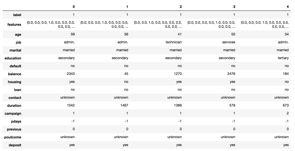
Figure 8
As you can see, we now have features column and label column.
Randomly split data into train and test sets, and set seed for reproducibility.
train, test = df.randomSplit([0.7, 0.3], seed = 2018)
print(“Training Dataset Count: ” + str(train.count()))
print(“Test Dataset Count: ” + str(test.count()))
Training Dataset Count: 7764
Test Dataset Count: 3398
Logistic Regression Model
from pyspark.ml.classification import LogisticRegression
lr = LogisticRegression(featuresCol = ‘features’, labelCol = ‘label’, maxIter=10)
lrModel = lr.fit(train)
We can obtain the coefficients by using LogisticRegressionModel’s attributes.
import matplotlib.pyplot as plt
import numpy as np
beta = np.sort(lrModel.coefficients)
plt.plot(beta)
plt.ylabel(‘Beta Coefficients’)
plt.show()
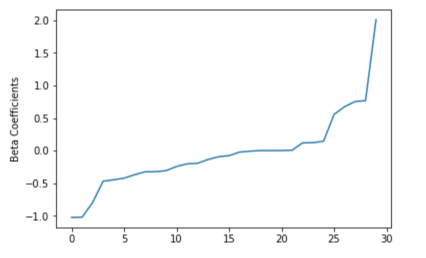
Figure 9
Summarize the model over the training set, we can also obtain the receiver-operating characteristic and areaUnderROC.
trainingSummary = lrModel.summary
roc = trainingSummary.roc.toPandas()
plt.plot(roc[‘FPR’],roc[‘TPR’])
plt.ylabel(‘False Positive Rate’)
plt.xlabel(‘True Positive Rate’)
plt.title(‘ROC Curve’)
plt.show()
print(‘Training set areaUnderROC: ‘ + str(trainingSummary.areaUnderROC))
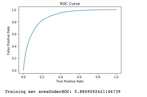
Figure 10
Precision and recall.
pr = trainingSummary.pr.toPandas()
plt.plot(pr[‘recall’],pr[‘precision’])
plt.ylabel(‘Precision’)
plt.xlabel(‘Recall’)
plt.show()
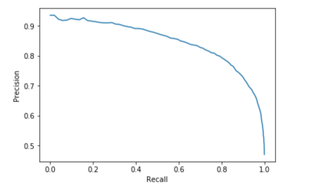
Figure 11
Make predictions on the test set.
predictions = lrModel.transform(test)
predictions.select(‘age’, ‘job’, ‘label’, ‘rawPrediction’, ‘prediction’, ‘probability’).show(10)
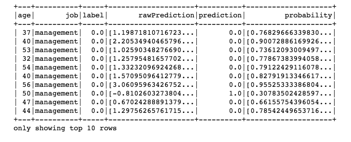
Figure 12
Evaluate our Logistic Regression model.
from pyspark.ml.evaluation import BinaryClassificationEvaluator
evaluator = BinaryClassificationEvaluator()
print(‘Test Area Under ROC’, evaluator.evaluate(predictions))
Test Area Under ROC 0.8858324614449619
Decision Tree Classifier
Decision trees are widely used since they are easy to interpret, handle categorical features, extend to the multi-class classification, do not require feature scaling, and are able to capture non-linearities and feature interactions.
from pyspark.ml.classification import DecisionTreeClassifier
dt = DecisionTreeClassifier(featuresCol = ‘features’, labelCol = ‘label’, maxDepth = 3)
dtModel = dt.fit(train)
predictions = dtModel.transform(test)
predictions.select(‘age’, ‘job’, ‘label’, ‘rawPrediction’, ‘prediction’, ‘probability’).show(10)
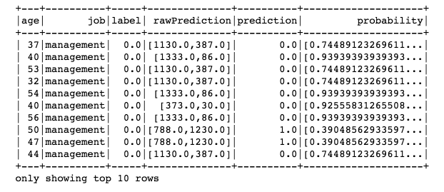
Figure 13
Evaluate our Decision Tree model.
evaluator = BinaryClassificationEvaluator()
print(“Test Area Under ROC: ” + str(evaluator.evaluate(predictions, {evaluator.metricName: “areaUnderROC”})))
Test Area Under ROC: 0.7807240050065357
One simple decision tree performed poorly because it is too weak given the range of different features. The prediction accuracy of decision trees can be improved by Ensemble methods, such as Random Forest and Gradient-Boosted Tree.
Random Forest Classifier
from pyspark.ml.classification import RandomForestClassifier
rf = RandomForestClassifier(featuresCol = ‘features’, labelCol = ‘label’)
rfModel = rf.fit(train)
predictions = rfModel.transform(test)
predictions.select(‘age’, ‘job’, ‘label’, ‘rawPrediction’, ‘prediction’, ‘probability’).show(10)
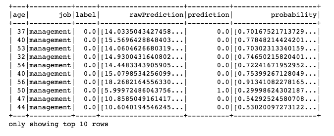
Figure 14
Evaluate our Random Forest Classifier.
evaluator = BinaryClassificationEvaluator()
print(“Test Area Under ROC: ” + str(evaluator.evaluate(predictions, {evaluator.metricName: “areaUnderROC”})))
Test Area Under ROC: 0.8846453518867426
Gradient-Boosted Tree Classifier
from pyspark.ml.classification import GBTClassifier
gbt = GBTClassifier(maxIter=10)
gbtModel = gbt.fit(train)
predictions = gbtModel.transform(test)
predictions.select(‘age’, ‘job’, ‘label’, ‘rawPrediction’, ‘prediction’, ‘probability’).show(10)
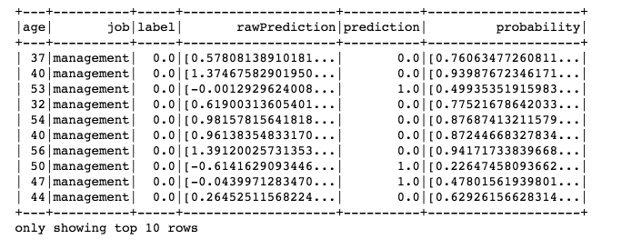
Figure 15
Evaluate our Gradient-Boosted Tree Classifier.
evaluator = BinaryClassificationEvaluator()
print(“Test Area Under ROC: ” + str(evaluator.evaluate(predictions, {evaluator.metricName: “areaUnderROC”})))
Test Area Under ROC: 0.8940728473145346
Gradient-Boosted Tree achieved the best results, we will try tuning this model with the ParamGridBuilder and the CrossValidator. Before that we can use explainParams() to print a list of all params and their definitions to understand what params available for tuning.
print(gbt.explainParams())
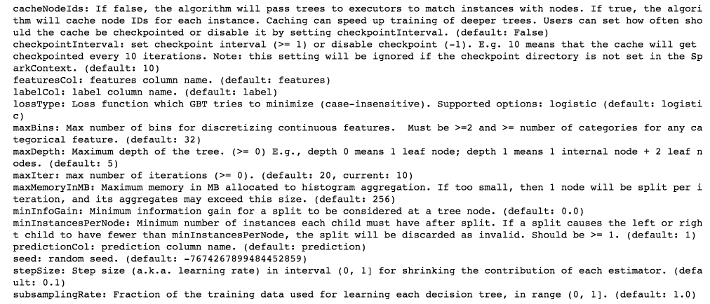
Figure 16
from pyspark.ml.tuning import ParamGridBuilder, CrossValidator
paramGrid = (ParamGridBuilder()
.addGrid(gbt.maxDepth, [2, 4, 6])
.addGrid(gbt.maxBins, [20, 60])
.addGrid(gbt.maxIter, [10, 20])
.build())
cv = CrossValidator(estimator=gbt, estimatorParamMaps=paramGrid, evaluator=evaluator, numFolds=5)
# Run cross validations. This can take about 6 minutes since it is training over 20 trees!
cvModel = cv.fit(train)
predictions = cvModel.transform(test)
evaluator.evaluate(predictions)
0.8981050997838095
To sum it up, we have learned how to build a binary classification application using PySpark and MLlib Pipelines API. We tried four algorithms and gradient boosting performed best on our data set.
Source code can be found on Github.