
Ready to learn Machine Learning? Browse Machine Learning Training and Certification courses developed by industry thought leaders and Experfy in Harvard Innovation Lab.
A way to teach Machines how to comprehend Natural Languages.
Introduction
Humans don’t start their thinking from scratch every second. As you read this essay, you understand each word based on your understanding of previous words. You don’t throw everything away and start thinking from scratch again. Your thoughts have persistence.
Traditional neural networks can’t do this, and it seems like a major shortcoming. For example, imagine you want to classify what kind of event is happening at every point in a movie. It’s unclear how a traditional neural network could use its reasoning about previous events in the film to inform later ones.
Recurrent neural networks address this issue. They are networks with loops in them, allowing information to persist.
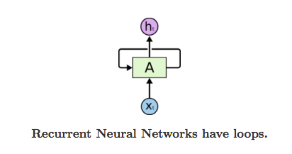
In the above diagram, a chunk of neural network, A, looks at some input xt and outputs a value ht. A loop allows information to be passed from one step of the network to the next. A recurrent neural network can be thought of as multiple copies of the same network, each passing a message to a successor.Consider what happens if we unroll the loop:
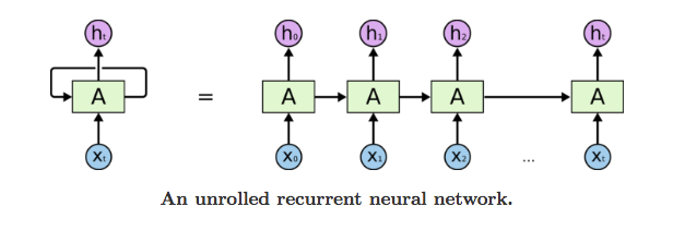
This chain-like nature reveals that recurrent neural networks are intimately related to sequences and lists. They’re the natural architecture of neural network to use for such data. And they certainly are used! In the last few years, there have been incredible success applying RNNs to a variety of problems: speech recognition, language modeling, translation, image captioning… The list goes on.
Although it is not mandatory but it would be good for the reader to understand what WordVectors are. Here’s my earlier blog on Word2Vec, a technique to create Word Vectors.
What is Recurrent Neural Networks
A glaring limitation of Vanilla Neural Networks (and also Convolutional Networks) is that their API is too constrained: they accept a fixed-sized vector as input (e.g. an image) and produce a fixed-sized vector as output (e.g. probabilities of different classes). Not only that: These models perform this mapping using a fixed amount of computational steps (e.g. the number of layers in the model).
The core reason that recurrent nets are more exciting is that they allow us to operate over sequences of vectors: Sequences in the input, the output, or in the most general case both.
A few examples may make this more concrete:
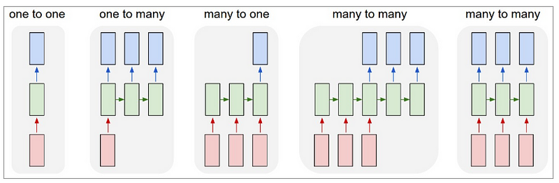
Each rectangle is a vector and arrows represent functions (e.g. matrix multiply). Input vectors are in red, output vectors are in blue and green vectors hold the RNN’s state (more on this soon). From left to right:
- Vanilla mode of processing without RNN, from fixed-sized input to fixed-sized output (e.g. image classification).
- Sequence output (e.g. image captioning takes an image and outputs a sentence of words).
- Sequence input (e.g. sentiment analysis where a given sentence is classified as expressing positive or negative sentiment)
- Sequence input and sequence output (e.g. Machine Translation: an RNN reads a sentence in English and then outputs a sentence in French).
- Synced sequence input and output (e.g. video classification where we wish to label each frame of the video).
Notice that in every case are no pre-specified constraints on the lengths sequences because the recurrent transformation (green) is fixed and can be applied as many times as we like.
We’ll see in a bit, RNNs combine the input vector with their state vector with a fixed (but learned) function to produce a new state vector.
RNN Computation
So how do these things work?
They accept an input vector x and give an output vector y. However, crucially this output vector’s contents are influenced not only by the input you just fed in, but also on the entire history of inputs you’ve fed in in the past. Written as a class, the RNN’s API consists of a single step function:
rnn = RNN()

y = rnn.step(x) # x is an input vector, y is the RNN’s output vector
The RNN class has some internal state that it gets to update every time step is called. In the simplest case this state consists of a single hidden vector h. Here is an implementation of the step function in a Vanilla RNN:
# …
def step(self, x):
# update the hiddenstate
self.h = np.tanh(np.dot(self.W_hh, self.h) + np.dot(self.W_xh, x))
# compute the output vector
y = np.dot(self.W_hy, self.h)
The above specifies the forward pass of a vanilla RNN. This RNN’s parameters are the three matrices –
- W_hh : Matrix based on the Previous Hidden State
- W_xh : Matrix based on the Current Input
- W_hy : Matrix based between hidden state and output
The hidden state self.h is initialized with the zero vector. The np.tanh(hyperbolic tangent) function implements a non-linearity that squashes the activations to the range [-1, 1].
So how it works-
There are two terms inside of the tanh: one is based on the previous hidden state and one is based on the current input. In numpy np.dot is matrix multiplication. The two intermediates interact with addition, and then get squashed by the tanh into the new state vector.
The Math notation for the hidden state update is –
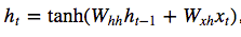
where tanh is applied elementwise.
We initialize the matrices of the RNN with random numbers and the bulk of work during training goes into finding the matrices that give rise to desirable behavior, as measured with some loss function that expresses your preference to what kinds of outputs y you’d like to see in response to your input sequences x
Now going deep –
y1 = rnn1.step(x)
y = rnn2.step(y1)
In other words we have two separate RNNs: One RNN is receiving the input vectors and the second RNN is receiving the output of the first RNN as its input. Except neither of these RNNs know or care — it’s all just vectors coming in and going out, and some gradients flowing through each module during backpropagation.
I’d like to briefly mention that in practice most of us use a slightly different formulation than what I presented above called a Long Short-Term Memory (LSTM) network. The LSTM is a particular type of recurrent network that works slightly better in practice, owing to its more powerful update equation and some appealing backpropagation dynamics. I won’t go into details, but everything I’ve said about RNNs stays exactly the same, except the mathematical form for computing the update (the line self.h = … ) gets a little more complicated. From here on I will use the terms “RNN/LSTM” interchangeably but all experiments in this post use an LSTM.
We will cover LSTM in a separate blog.
An Example — Character-Level Language Models
We’ll train RNN character-level language models. That is, we’ll give the RNN a huge chunk of text and ask it to model the probability distribution of the next character in the sequence given a sequence of previous characters. This will then allow us to generate new text one character at a time.
As a working example, suppose we only had a vocabulary of four possible letters “helo”, and wanted to train an RNN on the training sequence “hello”. This training sequence is in fact a source of 4 separate training examples:
- The probability of “e” should be likely given the context of “h”
- “l” should be likely in the context of “he”
- “l” should also be likely given the context of “hel”
- “o” should be likely given the context of “hell”
Concretely, we will encode each character into a vector using 1-of-k encoding (i.e. all zero except for a single one at the index of the character in the vocabulary), and feed them into the RNN one at a time with the help of a step function. We will then observe a sequence of 4-dimensional output vectors (one dimension per character), which we interpret as the confidence the RNN currently assigns to each character coming next in the sequence. Here’s a diagram:
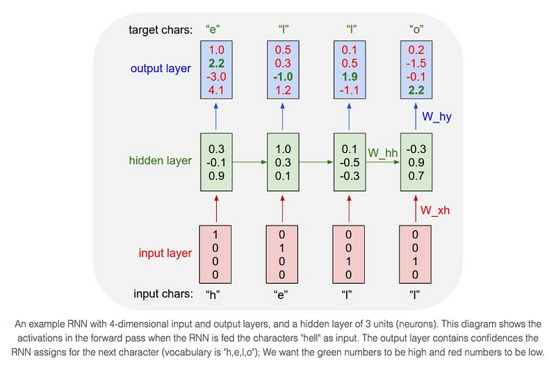
For example, we see that in the first time step when the RNN saw the character “h” it assigned confidence of 1.0 to the next letter being “h”, 2.2 to letter “e”, -3.0 to “l”, and 4.1 to “o”. Since in our training data (the string “hello”) the next correct character is “e”, we would like to increase its confidence (green) and decrease the confidence of all other letters (red). Similarly, we have a desired target character at every one of the 4 time steps that we’d like the network to assign a greater confidence to.
Since the RNN consists entirely of differentiable operations we can run the back-propagation algorithm (this is just a recursive application of the chain rule from calculus) to figure out in what direction we should adjust every one of its weights to increase the scores of the correct targets (green bold numbers).
We can then perform a parameter update, which nudges every weight a tiny amount in this gradient direction. If we were to feed the same inputs to the RNN after the parameter update we would find that the scores of the correct characters (e.g. “e” in the first time step) would be slightly higher (e.g. 2.3 instead of 2.2), and the scores of incorrect characters would be slightly lower.
We then repeat this process over and over many times until the network converges and its predictions are eventually consistent with the training data in that correct characters are always predicted next.
A more technical explanation is that we use the standard Softmax classifier (also commonly referred to as the cross-entropy loss) on every output vector simultaneously. The RNN is trained with mini-batch Stochastic Gradient Descent and I like to use RMSProp or Adam (per-parameter adaptive learning rate methods) to stabilize the updates.
Notice also that the first time the character “l” is input, the target is “l”, but the second time the target is “o”. The RNN therefore cannot rely on the input alone and must use its recurrent connection to keep track of the context to achieve this task.
At test time, we feed a character into the RNN and get a distribution over what characters are likely to come next. We sample from this distribution, and feed it right back in to get the next letter. Repeat this process and you’re sampling text!