Ready to learn Machine Learning?Browse Machine Learning Training and Certification courses developed by industry thought leaders and Experfy in Harvard Innovation Lab.
This is the 3rd article of series “Coding Deep Learning for Beginners”. Here, you will find links to the 1st article and the 2nd article.
Why Linear Regression?
Some of you may wonder, why the article series about explaining and coding Neural Networks starts with basic Machine Learning algorithm such as Linear Regression. It’s very justifiable to start from there. First of all, it is a very plain algorithm so the reader can grasp an understanding of fundamental Machine Learning concepts such as Supervised Learning, Cost Function, and Gradient Descent. Additionally, after learning Linear Regression it is quite easy to understand Logistic Regression algorithm and believe or not — it is possible to categorise that one as small Neural Network. You can expect all of those and even more covered in few next articles!
Tools
Let’s introduce the most popular libraries that can be found in every Python based Machine Learning or Data Science related project.
- NumPy — a library for scientific computing, perfect for Multivariable Calculus & Linear Algebra. Provides ndarray class which can be compared to Python list that can be treated as vector or matrix.
- Matplotlib — toolkit for data visualisation, allows to create various 2d and 3d graphs.
- Pandas—this library is a wrapper for Matplotlib and NumPy libraries. It provides DataFrame class. It treats NumPy matrices as tables, allowing access to rows and columns by their attached names. Very helpful in data loading, saving, wrangling, and exploration process. Provides an interface of functions that makes deployment faster.
Each library can be installed separately with using Python PyPi. They will be imported in code of every article under following aliases.
What is Linear Regression?
It’s a Supervised Learning algorithm which goal is to predict continuous, numerical values based on given data input. From the geometrical perspective, each data sample is a point. Linear Regression tries to find parameters of the linear function, so the distance between the all the points and the line is as small as possible. Algorithm used for parameters update is called Gradient Descent.
Training of Linear Regression model. The left graph displays the change of linear function parameters over time. The plot on the right renders the linear function using current parameters (source: Siraj Raval GitHub).
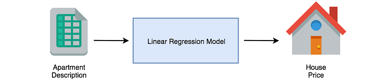
For example, if we have a dataset consisting of apartments properties and their prices in some specific area, Linear Regression algorithm can be used to find a mathematical function which will try to estimate the value of different apartment (outside of the dataset), based on its attributes.
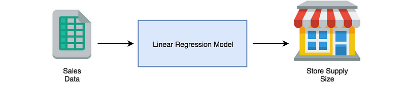
Another example can be a prediction of food supply size for the grocery store, based on sales data. That way the business can decrease unnecessary food waste. Such mapping is achievable for any correlated input-output data pairs.
Data preparation
Before coding Linear Regression part, it would be good to have some problem to solve. It is possible to find a lot of datasets on websites like UCI Repositoryor Kaggle. After going through many of those, none was suitable for study case of this article.
In order to get data, I’ve entered Polish website dominium.pl, which is a search engine for apartments in Cracow city — area where I live. I have entirely randomly chosen 76 apartments, written down their attributes and saved to the .csv file. The goal was to train Linear Regression model capable of predicting apartments prices in Cracow.
Dataset is available on my Dropbox under this link.
Loading data
Let’s start by reading data from the .csv file to DataFrame object of Pandas and displaying a few data rows. To achieve that read_csv function will be used. Data is separated with colon character which is why sep="," parameter was added. Function head renders first five rows of data in the form of the pleasantly readable HTML table.
The output of the code looks as following:
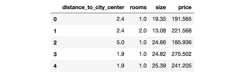
DataFrame visualisation in Jupyter Notebook.
As presented in the table, there are four features describing apartment properties:
- distance_to_city_center – distance from dwelling to Cracow Main Squareon foot, measured with Google Maps,
- rooms – the number of rooms in the apartment,
- size – the area of the apartment measured in square meters,
- price – target value (the one that needs to be predicted by model), cost of the apartment measured in Polish national currency—złoty.
Visualising data
It is very important to always understand the structure of data. The more features there are, the harder it is. In this case, scatter plot is used to display the relationship between target and training features.
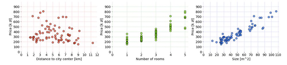
Charts show whole data from cracow_apartments.csv. It was prepared with Matplotlib library in Jupyter Notebook. The code used to create these charts can be found under this link.
Depending on what is necessary to show, some other types of visualization (e.g. box plot) and techniques could be useful (e.g. clustering). Here, a linear dependency between features can be observed — with the increase of values on axis x, values on the y-axis are linearly increasing or decreasing accordingly. It’s great because if that was not the case (e.g. relationship would be exponential), then it would be hard to fit a line through all the points and different algorithm should be considered.
Formula
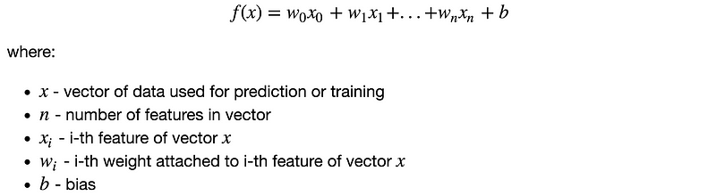
The Linear Regression model is a mathematical formula that takes vector of numerical values (attributes of single data sample) as an input and uses them to make a prediction.
Mapping the same statement in the context of the presented problem, there are 76 samples containing attributes of Cracow apartments where each sample is a vector from mathematical perspective. Each vector of features is paired with target value (expected result from formula).

According to the algorithm, every feature has a weight parameter assigned. It represents it’s importance to the model. The goal is to find the values of weights so the following equation is met for every apartment data.

The left side of the equation is a linear function. As manipulation of weight values can change an angle of the line. Although, there is a still one element missing. Current function is always going through (0,0) point of the coordinate system. To fix that, another trainable parameter is added.

The parameter is named bias and it gives the formula a freedom to move on the y-axis up and down.
The purple parameters belong to the model and are used for prediction for every incoming sample. That’s why finding a solution that works best for all samples is necessary. Formally the formula can be written as:
Initialization
It’s a phase where the first version of a model is created. Model after initialization can already be used for prediction but without training process, the results will be far from good. There are two things to be done:
- create variables in code that represents weights and bias parameters,
- decide on starting values of model parameters.
Initial values of model parameters are very crucial for Neural Networks. In case of Linear Regression parameter values can be set to zero at the start.
Function init(n) returns a dictionary containing model parameters. According to the terminology presented in the legend below the mathematical formula, n is the number of features used to describe data sample. It is used by zeros function of NumPy library, to return a vector of ndarray type with n elements and zero value assigned to each. Bias is a scalar set to 0.0 and it is a good practice to keep the variables as floats rather than integers. Both weights and bias are accessible under “w” and “b” dictionary keys accordingly.
For Cracow apartment dataset there are three features describing each sample. Here is the result of calling init(3) :

Prediction
Created model parameters can be used by the model for making a prediction. The formula has been already shown. Now it’s time to turn it into the Python code. First, every feature has to be multiplied by its corresponding weight and summed up. Then bias parameter needs to be added to the product of the previous operation. The outcome is a prediction.
Function predict(x, parameters) takes two arguments:
- vector
xof features representing a data sample (e.g. single apartment), - Python dictionary
parameterswhich stores parameters of the model along with their current state.
Assemble
Let’s put together all code parts that were created and display at the results.
Only one feature was used for prediction what reduced formula to form:

This was intentional as displaying results on the data which has more than 1–2–3 dimensions becomes troublesome, unless Dimensionality Reductiontechniques are used (e.g. PCA). From now on, for learning purposes all code development will be done only on size feature. When Linear Regression code will be finished, results with usage of all features will be presented.
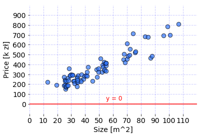
Line used to fit the data by Linear Regression model with current parameters. Code for visualisation is available under this link.
The model parameters were initialized with zero values which means that the output of the formula will always be equal to zero. Consequently, the prediction is a Python list of 76 zero values which are predicted prices for each apartment separately. But that’s ok for now. Model behavior will improve after training with the Gradient Descent is used and explained.
Bonus takeouts from the code snippet are:
- Features to be used by model and target value were stored in
featuresandtargetPython lists. Thanks to that there is no need to modify the whole code if a different set of features should be used. - It is possible to parse DataFrame object to ndarray by using as_matrixfunction.
Summary
In this article, I have introduced the tools that I am going to use in the whole article series. Then I have presented the problem I am going to solve with Linear Regression algorithm. At the end, I have shown how to create Linear Regression model and use it for making a prediction.
In the next article I will explain how to compare sets of parameters and measure model performance. Finally, I will show how to update model parameters with Gradient Descent algorithm.